Bayesian Language
I have tried to conquer Bayesian modeling several times since 2010; read a lot paper, couple of books, and took some online classes. Yes, you can remember math terms, you may follow what they say in the paper while you are reading it, you may even be able to derive the equations just as they do. But what's hard is to really understand what's going on behind those equations, without which you are bound to forget what you think you know after a certain period. Then you might need to repeat the learning process, however only to find you stuck in a loop.
That's because there is a Bayesian language and a way to think about relationships in data, which is very different from deterministic modeling such as Neural Networks. Natually, there should be a way to link every concept in Bayesian to Neural Networks. After all they both are trying to solve the same set of problems (regression and classification) by slightly different ways. Also, as we have already seen in the previous post, VAE can be expressed as a Neural Network. People have already done a lot of research to link the two, another example being the linkage of Gaussian Naive Bayes classifier and logistic regression. (from Andrew Ng)
Let's start one step at a time. As usual, notations first. Very often, I would ignore the notation part when reading any paper (because it is boring for sure). But please read it this time, not only because these are building characters of this new language we are getting into, but also it could be a nice recollection of certain basic concepts from high school probability. Here's a refresher I found very useful myself.
Notations
- Uppercase \(X\) denotes a random variable. Different with deterministic variable, random variable does not have a fixed value, but several possible values with probabilities.
- Uppercase \(P(X)\) denotes the probability distribution over that variable. We can say \(P(X) \sim N(0,1)\), which means this random variable generates value under a standard normal distribution.
- Lowercase \(x \sim P(X)\) denotes a value \(x\) sampled from the probability distribution \(P(X)\) via some generative process.
- Lowercase \(p(X)\) is the density function of the distribution of \(X\). It is a scalar function over the measure space \(X\).
- \(p(X=x)\) (shorthand \(p(x)\)) denotes the density function evaluated at a particular value \(x\).
Now, let's take a look at the first step. Normally, we are trying to model a dataset from a probability view. For example, we have an image of cat. The pixels in the image is our data (observation variable \(X\) in probability view). We believe this observable variable is generated from a hidden (latent) variable \(Z\), which can be a binary variable (cat or non-cat). We can draw this relationship via the following graph:
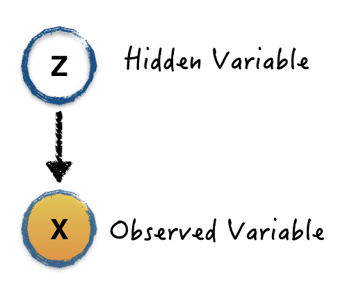
The edge drawn from \(Z\) to \(X\) relates the two variables together via the conditional distribution \(P(X | Z)\). Now, it's important to jump out of the graph and conditional probability, to think about the problem we try to solve, which is: given the image, is this an image of cat or not? In the probability language, what's the conditional probability \(P(Z|X)\)? Even if we modeled the graph, what we got is the \(P(X|Z)\), how can we get to the problem we are interested? Bayesian comes to play here.
\[ p(Z|X)=\frac{p(X|Z)p(Z)}{p(X)} \]
Let's assume we can model the graph \(p(X|Z)\) somehow. We can get the final answer if we got \(p(Z)\) and \(p(X)\). In Bayesian Language, we have some names for all those math terms. They are just names, but would help you to read paper and discuss with "experts".
Bayesian Language
- \(p(Z|X)\) is the posterior probability. This is the most important term in Bayesian modeling, because this is the question we are interested.
- This \(p(X|Z)\) is the likelihood. It means given the hidden variable \(Z\), how likely it generates observed images as we have seen in training data. Building this is building the graph. The famous term "maximum likelihood estimation" is one way to solve this. It tries to find the best hidden variable \(Z\) to lead to good likelihood.
- \(p(Z)\) is the prior probability. This captures any prior information we know about \(Z\) - for example, if we think that \(\frac{1}{3}\) of all images in existence are of cats, then \(p(Z=1)=\frac{1}{3}\) and \(p(Z=0)=\frac{2}{3}\)
- \(p(X)\) is called model evidence or marginal likelihood. The way to compute this is marginalizing the likelihood over hidden variable \(Z\).
- \(p(X) = \intdz\)
- Marginalization is the bread and butter of Bayesian modeling, because this gives us the model uncertainty.
This is the Bayesian language. It's easy to follow, but too abstract to understand, right? Because everything here is probability, but not straight-forward equations that we can code up. I agree, and feel the same pain. Now, let's visualize it through a simple example under Naive Bayesian Classifier.
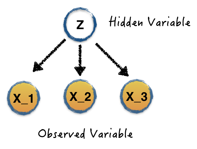
This is the structure graph of Naive Bayesian classifier. Very similar to the previous graph, but with one assumption, all the observations are conditional independent given the hidden variable. Let's say we have 3 observed binary variables \(X_1\), \(X_2\) and \(X_3\) and one binary hidden variable \(Z=\{0,1\}\). Given a dataset containing the pairs of values of observed variables and hidden variables, \(
As we have shown above, in order to solve the posterior probability, we need to learn the likelihood \(p(X|Z)\), the prior \(p(Z)\) and the model evidence \(p(X)\).
It's easy to get the prior \(p(Z=1)\), just estimate it from counting cases in the training data
\[ p(Z=1) = \frac{\#Z==1}{\#Total} \]
The hard part is the likelihood, \(p(X_1=x_1,X_2=x_2,X_3=x_3|Z=1)\), which is a conditional joint probability. Thanks to the independence assumption of Naive Bayes, we can write this likelihood like this:
\[ p(X_1=x_1,X_2=x_2,X_3=x_3|Z=1) = p(X_1=x_1|Z=1)p(X_2=x_2|Z=1)p(X_3=x_3|Z=1) \]
Compute the conditional probability with one variable is easy:
\[ p(X_i|Z)=\frac{P(X_i\cap Z)}{P(Z)}=\frac{\#(X_i \& Z)}{\#(Z)} \]
The model evidence is just an integral of those posteriors.
Now, hopefully we have a clear picture how Bayes model works. Keep in mind, the posterior is easy under the Naive Bayes assumptions, but hard ('nontrackable') in most cases. You can imagine it being even harder to compute model evidence in those cases (because of the integral).
Till now, I guess you may have the same question as I have. The "hidden variable" is our target, which is observable in the training data. Many situations, the real "hidden variable" is the variables we do not even know in the training data, such as some object features in the image. How can we define this kind of a problem? How can we present them with the graph?
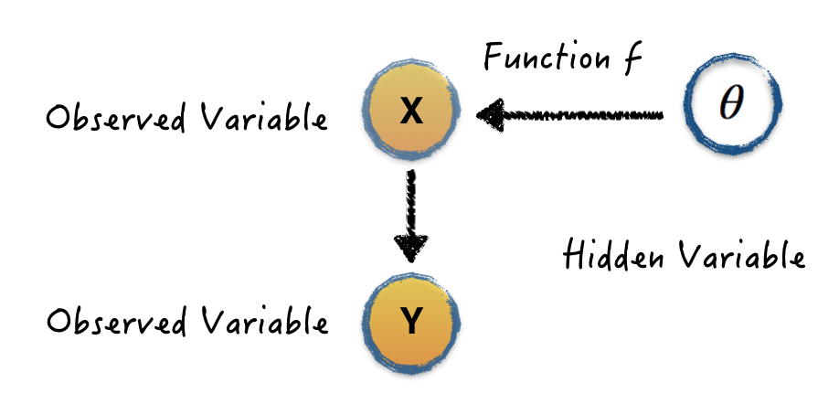
This is a graph that defines a more complicated but real-life problem. Given the training inputs \(X=\{x_1,...,x_N\}\) and their corresponding outputs \(Y=\{y_1,...,y_N\}\), in Bayesian (parametric) modeling, we would like to find the parameters \(\theta\) of a function \(y=f^{\theta}(x)\) that is likely to have generated our outputs. In another word, what parameters are likely to have generated our data?
The model forward (testing/inference) is not the posterior probability anymore. Given a new input point \(x'\) and the training data, we would like to infer what's the probability of corresponding value of \(y'\)
\[ p(y'|x', X, Y) = \int{p(y|x', \theta)p(\theta|X,Y)d\theta} \]
It can also be written as
\[ p(y'|x', X, Y) = \int{f_{\theta}(x')p(\theta|X,Y)d\theta} \]
We can see that is is marginalizing likelihood over posterior. Also remember, in the Bayesian modeling, \(\theta\) is not one best value found, but rather a set of possible values with corresponding probabilities. Comparing with the "Bayesian Language" shown above, we need to slightly modify the language definition.
Bayesian Language Update
- Posterior Probability \(p(\theta|X,Y) = \frac{p(Y|X,\theta)p(\theta)}{p(Y|X)}\)
- Likelihood \(p(Y|X,\theta)\)
- Prior Probability \(p(\theta)\)
- Model Evidence \(p(Y|X) = \int{p(Y|X,\theta)p(\theta)d\theta}\)
The same as previous examples, the most important part is still the posterior \(p(\theta|X,Y)\). It cannot usually be evaluated analytically. Instead we seek some estimations such as MC based sampling method or by an approximating variational distribution.
One more point I need to make here is, the output of Bayesian inference is not just a value, but expected values and uncertainties. If we deal with the regression problem, the inference can be express as Gaussian likelihood.
\[ \mathbf{E}(y') = \int{f_{\theta}(x')p(\theta|X,Y)d\theta} \]
\[ var(y') = \tau^{-1} I \]
If we deal with classification problem, the expectation is softmax likelihood. Yarin Gal described a way to extract prediction exception in a Bayesian view from Neural Network with dropout, which provides a good linkage between NN and Bayesian modeling.