Neural Network Infers Bayes
Congratulations, you have made to the third and final part! Equipped with the Bayesian language, we can start to look at the "special" regularization term in the VAE loss function and try to make sense of it. Most articles talk about "variational inference" and derive the equations of variational lower bound and KL divergence. I encourage you to read this blog from Eric Jang for more details of variational inference. In a different route, here we are going to focus on how to use Neural Networks to present Bayesian likelihood and posterior and how to setup the loss function. Let's start with our old friend, the directed graph of Bayesian modeling.
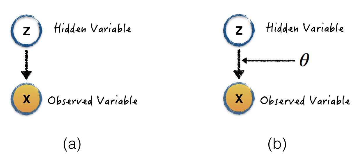
Graph (a) is the VAE we are interested in. Since VAE is a unsupervised model, what we want to learn is the hidden random variable \(Z\), which is a much lower representation of observed variable \(X\). This graph show us the posterior \(p(Z|X)\) is what we want to learn. Also, please keep in mind, the joint distribution \(p(X,Z)\) can be expressed as \(p(X|Z)P(Z)\) as shown in this graph. In order to compute the posterior distribution, Bayesian rule comes to convert it into likelihood, prior, and model evidence (the Bayesian language).
\[ p(Z|X)=\frac{p(X|Z)p(Z)}{p(X)} \]
Let's exam how to compute those terms one by one, starting from likelihood \(p(X|Z)\). As we discussed in last section, graph (b) means we can assume there is a function f with parameter \(\theta\) to generate the variable \(X\), and \(X\) is follows a Gaussian distribution. Then this likelihood can be expressed as Gaussian Likelihood (discussed in last section).
\[ p(X|Z) = p(X|Z,\theta) = N(X; f_{\theta}(Z), \tau^{-1}I) \]
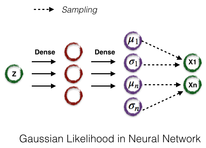
We can further assume \(tau^{-1}\) is a diagonal covariance matrix. If we use a neural network to present the function \(f_\theta\), this Gaussian likelihood can be expressed as this:
Through the famous reparametrization trick , we can use gradient descent to learn the NN weights \(\theta\) with sampling given a set of training samples with \(Z\) and corresponding \(X\)
In order to compute the posterior distribution, likelihood is not enough. The hardest term is computing model evidence \(p(X)\), which is an integral over all configuration of hidden variables.
\[ p(X) = \int{p(X|Z)p(Z)dz} \]
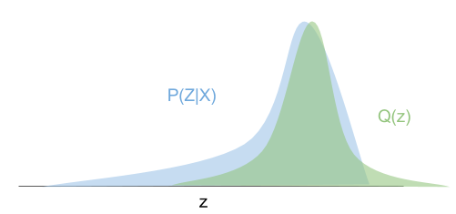
It requires us to consider all possible of hidden variables, in another word, we need to train tons of neural networks, which is untraceable. Sampling is one way to solve this. It means instead of evaluate all possible hidden variable configurations, we can compute some of them by sampling, but it is still very slow. The way VAE deal with this is called variational inference. It says we can try to learn a simple posterior which is easy to compute, and make it similar to the true posterior.
\[ q(Z|X,\lambda) = p(Z|X,\theta) \]
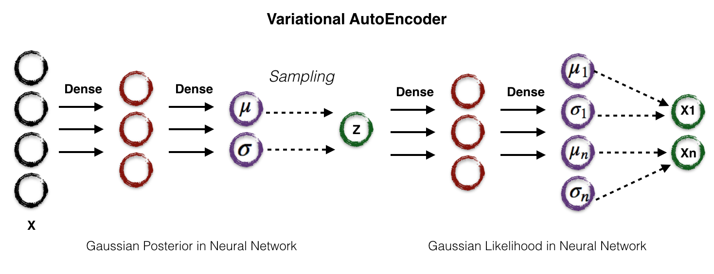
We can assume distribution \(q(Z|X,\lambda)\) is a multivariate Gaussian. We can visualize this concept by the following graph.
Assuming the approximation distribution \(q\) is Gaussian, we can use similar technique (compute the Gaussian likelihood). The neural network can be like this:
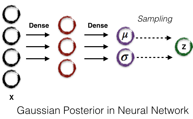
The Gaussian posterior neural network serves as the encoder network, and Gaussian likelihood neural network serves as the decoder network. Putting them all together, we can get the VAE network shown in section 1.
The last bit is how to define our loss function for this VAE network. As we described above, we need to make the approximation distribution \(q\) similar to the true posterior, very straight-forward, Kullback-Leibler (KL) divergence is our loss. Let's take a look at KL divergence definition now:
\[ KL(q(Z|X,\lambda)||p(Z|X)) = E_q[log{q(Z|X,\lambda)}] - E_q[log{p(X,Z)} + log{p(X)}] \]
The beauty of this equation is hard rock posterior \(p(Z|X)\) is gone. But wait a minute, the monster term \(p(X)\) comes back! Do we still need to deal with this endless integral? The answer is no, we can use some math trick to get rid of it. Let me show you the trick. Firstly, we group the first and second term in KL divergence together (times \(-1\)) and call it Evidence Lower Bound (ELBO).
\[ ELBO(\lambda) = E_q[log{p(X,Z)} - E_q[log{q(Z|X,\lambda)}] \]
Then rewrite the KL divergence using \(ELBO(\lambda)\)
\[KL = log{p(X) - ELBO}\]
In order to maximize \(KL\), we can just minimize \(ELBO\) instead, since \(KL\) is always positive by definition.
Through some math re-writing, we can get the final loss function as negative of \(ELBO\)
\[loss = KL(q(Z|X,\theta)||p(Z)) - log{p(X|Z,\lambda)}\]
\(log{p(X|Z,\lambda)}\) is the binary cross-entropy we used as in AutoEncoder, and \( KL(q(Z|X,\theta)||p(Z)) \) is the regularization term.