Gaussian Process (GP) is Easy to Understand
In the beginning
This is a follow-up blog of "Variantial AntoEncoder", in which I tried to explain VAE in a Neural Network way before relating it to Bayesian machine learning. As we know, VAE is a unsupervised learning method; now, I will try to explain the most important supervised learning method in Bayesian machine learning, called Gaussian Process.
I have tried many many times to understand GP in different ways, through papers, books, videos, and had even written my own GP software in Theano. I found most materials starting with a GP definition such as "A Gaussian process defines a distribution over functions has multivariate Gaussian distribution", which I cannot understand for a very long time. What is the distribution of functions? What does it looks like? They also talk about the so-called "covariance function". How does those functions present the "covariance"? In our normal people's mind, "covariance" is not defined as some sort of wierd function, but just an average of squared residuals as shown in Wikipedia
In this blog, I try to make sense all those definitions. We do need some linear algebra knowledge; if you are not familar with it, I find Goodfellow's book chapter very helpful.
This blog explains Gaussian Process in Bayesian language. If you are not familar with it, please read my previous blog Bayesian Language.
Linear Regression
I assume everyone is familiar with linear regression, which is the reason I start with linear regression. Actually, Gaussian Process originates from it; it is just an elaboration of it from a Bayesian view. I have a somewhat personal preference of building models that might eventually become complex from the very simplest, and gradually increasing complexity. For example, (by profession I work in financial trading dealing with extremely noisy data,) I usually start with linear regression/classification or even simplier. Then if I want to include some more inputs, I extend it into multi-variate regression. Next if I find linear relationship is not enough to catch the phenomenon, I may generalize it to other functions such as Gaussian Process. If I want to catch the time-depdendencies in data, I can migrate the linear system into a state-space system. Somewhere in this growing process I may find my system too flexible in some sense (hard to learn), I could try adding some constrains (regularizations). In another words, we build a solution system by "+"-ing components and "-"-ing components (regularization), in the hope of finding a balanced point for a specific problem. Anyway, my point is we can understand GP better by expanding it from a simple linear regression.
Linear Regression with Point Estimation (Maximum Likelihood)
Given the training data \(X\in R^{n,m}\) (\(n\) samples with \(m\) features) and \(Y\in R^{n,1}\), the linear regression is looking for an "optimal" weight \(W, W \in R^{m,1}\) which fits the data well by the following linear model.
where \(\epsilon\) is a random noise following a Gaussian distribution,
\[ \epsilon \sim \mathcal{N}(0,\sigma^2) \]
Although it looks like an additional parameter \(\sigma\) is introduced, in the end we will see that it is actually irrelevant when deriving a point estimation solution. (It IS relevant, though, when deriving Bayesian solution.)
You may have heard the term "maximum likelihood" for getting an optimized solution. But what is likelihood? It measures how well the model fits the data given a set of weights, (or, how "likely" the output is generated by this model we proposed), which is the probability
\[ P(Y\mid X,w) = \prod_{i=1}^{n}p(y_i\mid x_i,w )=\prod_{i=1}^{n}\frac{1}{\sqrt{2\pi}\sigma}exp(-\frac{(y_i-x_i^Tw)^2}{2\sigma^2}) \]
The above simply says, because there is a Gaussian noise in modeling, each \(y\) comes out having a Gaussian distribution, therefore the collection of \(y\)'s, or \(Y\), can be written as a product of Gaussian distributions.
Through some simple linear algebra, we can get
\[ P(Y\mid X,w) \sim \mathcal{N}(X^Tw, \sigma^2I) \]
Simply taking the \(\log\) likelihood, we can get the following equation
\[ \log P(Y\mid X,w) = -n\log{\sigma} - \frac{n}{2}\log(2\pi) - \sum_{i=1}^{m}\frac{\parallel y_{*i}-y_i\parallel ^2}{2\sigma^2} \]
Maxmum likelihood is simply saying find me the \(w\) can get largest \(\log\) likelihood.
\[ argmax_{w}-\sum_{i=1}^{n}\frac{\parallel y_{*i}-y_i)\parallel ^2}{2\sigma^2} \]
Because we only want to find answers of \(w\), \(\sigma\) now is totally irrelevant. The numerator is all we care. Observe the numerator -- this is the same as minimizing mean square error! The solution is linear least square:
\[ w = (X^TX)^{-1}X^Ty \]
Linear Regression with Bayesian View
In a "point estimation" view, once we found the best weight to fit the data, story ends here. The final prediction given a new data \(X_*\) is
\[ Y_*=X_*^TW \]
But in a Bayesian view, we think all possible weights in our prior belief has a chance. The final prediction is a weighted average of all possible weight estimates. (Following: assume there are \(N\) possible weight matrices in our belief.)
\[ Y_* = \frac{1}{N}\sum_{j=1}^{N}\theta_j X_*^TW^j \]
The real world does not just have \(N\) scenarios. It has infinite. So we generalize with the sum rule in probability:
\[ P(y_*\mid x_*, X, y) = \int P(y_*\mid x_*, w)P(w \mid X, y) dw \]
As we have shown above, the first term is easy, which is a Gaussian distribution,
\[ P(y_*\mid x_*,w) \sim \mathcal{N}(x_*^Tw, \sigma^2I) \]
The second term is called posterior distribution. This gives us the weights of each possible \(w\). Think about this way, before we observe any data, we guess all possible \(w\) has equal chance. After we observed some data points, we changed our belief of the prior, and put some probability mass on some possible weights \(w\) which fits the data better. The changed distribution is called posterior distribution.
But how to compute this posterior distribution after observing training data? Bayesian Rule gives us the answer.
\[ P(w|y,X) = \frac{P(y\mid X, w)P(w)}{P(y\mid X)} \]
Through some linear algebra, we can get
\[ P(w|X, y) \sim \mathcal{N}(\frac{1}{\sigma^2}A^{-1}Xy, A^{-1}) \]
where
\[ A=\sigma^{-2}XX^T + \Sigma_p^{-1} \]
where our prior of \(w\) is
\[ w \sim \mathcal{N}(0, \Sigma_p^2) \]
This is called Bayesian Linear Regression. It gives us the predicted mean value as well as variance. The mean of posterior distribution looks similar to the point estimation, but with some extra terms. Actually, the extra term is proven the same as a \(L_2\) regularization in ridge regression. In another words, the Bayesian method gives us the regularization for free. That's why we can see many people saying Bayesian learning algorithms does NOT overfit data.
As you can see, the concept is simple, just a linear model expressed in Bayesian language. In order to get the equations, we just need to follow some rules in basic linear algebra. Now, I gonna show you it is also very easy to code and use it.
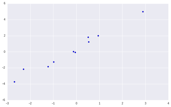
Let's generate some random 1-D random data.
# Generate data
X = np.random.uniform(-3., 3., (10,1))
X = np.hstack((X,np.ones((10,1))))
Y = np.dot(X,np.expand_dims(np.array([1.5,0.5]),1))+ np.random.randn(10,1) * 0.5
plt.scatter(X[:,0:1], Y)
The data looks like this.
After we set our prior distribution \(\mu_0, \Sigma_p\) and noise variance \(\sigma\) (shown in the following block), we can compute the posterior distributions from data.
# Set-up prior
sigma_n = 0.5
mu0 = np.zeros((2,1))
mu0[0,0] = 0.0
Sigma_p = np.identity(1)
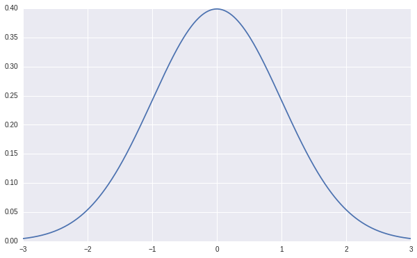
The prior we give to \(w\) is a normal distribution centered at \(0\) with \(\sigma=1\), it looks like this.
Computing the posterior is simplying saying we put some probability mass on some \(w\) values to fit the data. We can do that in 3 lines of code.
# Compute Posterior Distribution
A = sigma**(-2) * np.dot(X.T, X) + np.identity(1)
posterior_mu = sigma ** (-2) * np.dot(np.dot(np.linalg.inv(A), X.T),Y) +  np.dot(np.dot(np.linalg.inv(A), A), mu0)
posterior_var = np.linalg.inv(A)
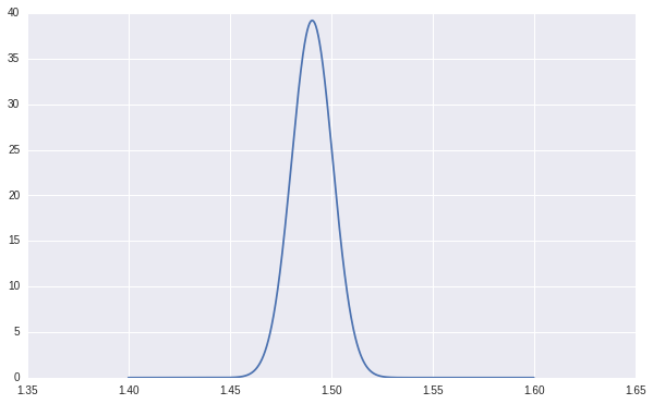
As shown in the following chart, our learned posterior distribution put a lot of probability mass around \(1.5\), which is our true \(w\) used to generate our random data.
If we use the learned posterior probabilities to make prediction, we can get the predicted \(y\) values along with our predictive variances. The code is also very straight-forward.
# Make predictions on test data
X_test = np.expand_dims(np.arange(-4,4,0.01),1)
X_test = np.hstack((X_test,np.ones((len(X_test),1))))
y_test_mu = sigma**(-2) * np.dot(np.dot(np.linalg.inv(A), X.T),Y) + np.dot(np.dot(np.linalg.inv(A), A), mu0)
y_test_mu = np.dot(X_test, y_test_mu)
y_test_var = np.dot(np.dot(X_test, np.linalg.inv(A)),X_test.T)
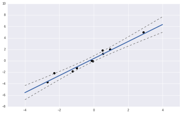
We can also plot the predicted values with \(+/- 3 \sigma\) lines.
Linear Regression Expansion with Basis Functions and Kernel Trick
The linear model looks good if we believe our data follows the linear relationship between input and output, but it's hard to catch any more complicated relationships. Remember in our Bayesian view of model prediction:
\[ P(y_*\mid x_*, X, y) = \int P(y_*\mid x_*, w)P(w \mid X, y) dw \]
We evaluate every possible \(w\) and weighted average them to make our final prediction. What if we consider every function instead of every weight? Then our prediction becomes to the weighted average of all possible functions.
\[ P(y_*\mid x_*, X, y) = \int P(y_*\mid x_*, \textbf{f})P(\textbf{f} \mid X, y) d\textbf{f} \]
The possible functions \(\textbf{f}\) can be \(
\[ Y=\sum_{j=1}^{M}\beta_j\phi_j(x) + \epsilon \]
The model is still a linear model, but it can catch nonlinear relationships through basis functions. This is called __linear regression with basis functions.
Given \(M\) basis functions \(\textbf{f}\), we are actually transformating the input space to a higher dimension feature space, and build a linear model on the high dimension feature space.
Let's look at the feature transformation in another way. We project the input data \(X\in R^{n, m}\) into feature data \(\hat{X} \in R^{n, M}\), where \(M >> m, M >> n\). If you still remember the basic linear algebra, the "fat" feature data has a lot of redundent features because \(n << M\). Then theoratically, there must be a way to define \(n\) functions, apply to the "sample dimension" and get exactly the same feature data. The function applies to samples \(K(.)=K(x_i,x_j)\) is called kernel function. This kernel function applies on data samples represents the covariance function. This trick is the famous kernel trick! It is also widely used in SVM. I won't derive the relationship between kernel function and basis function here, but here is the final relationship:
\[ K(x_i,x_j) = \sum_{m=1}^{M} \lambda_m \phi_m(x_i) \phi_m(x_j) + \delta_{ij}\sigma^2 \]
If we have infinite number of basis function, and make the prediction through Bayesian inference (the probability integral), we gets to Gaussian Process.
Gaussian Process
Prior and Covariance Function
As described above, Gaussian process is just a way to combine infinite possible basis functions to make a prediction through kernel trick. Maybe it's still too abstract to understand, let's look at it in a different way, which some people call it "Function-space view". Consider if we have a function \(\textbf{f}\); it maps 1-D input data to 1-D output data, \(y=\textbf{f}(x)\), which we do not know exactly the formula. But we know similar \(x\) values will generate similar \(y\) values; the similarity of \(y\) is defined by some distance function, \(k(x_p,x_q)\). For example:
\[ \textbf{similarity}(\textbf{f}(x_p), \textbf{f}(x_q)) = k(x_p,x_q) = \exp(-0.5\frac{\mid x_p - x_q \mid}{0.01} ^2) \]
This similarity function is called covariance function.
\[ \textbf{cov}(\textbf{f}(x_p), \textbf{f}(x_q)) = k(x_p,x_q) \]
How to relate covariance function to our familar sample covariance matrix? Let's take a look the following code! Given \(n\) numbers of \(x\), we can use the the covariance function to compute a sample covariance matrix for \(\textbf{f}(x)\), which is the sampled covariance matrix. If we assume the mean of \(y\) values are zero; given the sampled covariance matrix, we can generate the random samples of \(\textbf{f}(x)\).
def kernel(Xq, Xp):
return np.exp(-0.5 * (Xq - Xp.T)**2/0.01)
x = np.linspace(0., 1., 500) # 500 points of x
x = np.expand_dims(x,1)
cov_mat = kernel(x, x) # sample covariance matrix
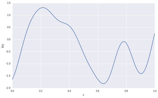
y = np.random.multivariate_normal(np.zeros((500)), cov_mat, 1) # generate random samples
The following figure shows the generated samples.
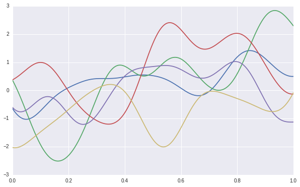
We can use the sampled covariance matrix to generate infinite \(y\) samples. As shown in the following figure, we have generate 5 sets of samples of \(y\). Each line presents a function, which are uncorrelated. With in each function, the \(y\) values are correlated according to the sampled covariance matrix. By this way, we can present infinite basis function, which is the prior of Gaussian process.
Posterior and Prediction
After observing some data, we can reject those function which does NOT fit the data. The remaining function gives us the prediction mean and variances. The following chart shows sampled 5 functions fits the data.
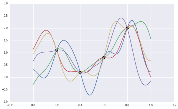
This trying-and-reject method is not efficient at all. Luckly, the Bayesian theory provides us a way to compute the posterior distribution easily and efficiently.
We know our posterior is a Gaussian distribution with covariance matrix defined by the covariance function.
\[ \textbf{f} \sim \mathcal{N}(0, K(X, X)) \]
The prediction is simply:
\[ P(y_*\mid x_*, X, y) = \int P(y_*\mid x_*, \textbf{f})P(\textbf{f} \mid X, y) d\textbf{f} \]
Through some linear algebra of multivariate Gaussian distribution, we can get the distribution of prediction as:
\[ \textbf{f}_* \mid X_*, X, f \sim \mathcal{N}(K(X_*, X)K(X,X)^{-1}\textbf{f}, K(X_*,X_*)-K(X_*,X)K(X,X)^{-1}K(X,X_*)) \]
Put it into code might be easiler to understand.
# After observing some data, compute the posterior distribution from prior.
X = np.expand_dims(np.array([0.2, 0.4, 0.6, 0.8]),1) # observed X
f = np.expand_dims(np.array([1.1, 0.2, 0.8, 2.0]),1) # observed Y

X_pred = np.expand_dims(np.linspace(0., 1., 500),1)
K = kernel(X,X)
K_inv = np.linalg.inv(K)
K_s = kernel(X_pred, X)
K_ss= kernel(X_pred, X_pred)
posterior_mu = np.dot(K_s, np.dot(K_inv, f))
posterior_covmat = K_ss - np.dot(K_s, np.dot(K_inv, K_s.T))
The Folowing code is used to generate samples from the learned posterior.
# Sample from the posterior distribution
sampled_f_pred = np.random.multivariate_normal(posterior_mu.flatten(), posterior_covmat, 5)

plt.scatter(X.flatten(), f.flatten(),s=100,color='k')
for i in range(len(sampled_f_pred)):
    plt.plot(X_pred.flatten(), sampled_f_pred[i,:])
Implementation Trick - Cholesky Decomposition
Until now, you should see how easy to understand and write your own Gaussian Process. You can use those couple of lines of code above to learn the posterior distribution and make predictions. You may notice in the equation and code above, we need to invert some covariance matrix, which can be tricky if data gets to large. Cholesky Decomposition is a simply trick to do the matrix inverse more efficiently. If you are not familar with it, you can read Section A.4 in the Gaussian Process book
Transfer it into compute code, here is the same code as we have shown above, but use Cholesky decompostion to compute the covariance matrix inverse.
# Cholesky Matrix Inverse
K = kernel(X,X)
K_inv = np.linalg.inv(K)
K_s = kernel(X_pred, X)
K_ss= kernel(X_pred, X_pred)
L = np.linalg.cholesky(K)
alpha = scipy.linalg.cho_solve((L,True), f)
V = scipy.linalg.cho_solve((L,True), K_s.T)
posterior_mu = np.dot(K_s, alpha)
posterior_covmat = K_ss - np.dot(K_s, V)
Research Topics
So, Gaussian Process is very straight-forward, right? Just some linear algebra with Bayesian rules. The ticky part is understanding the kernel trick and covariance function. Now, you may ask: Since it is so simply, why people use Deep Learning at all?
Firstly, Gaussian Process can be presented as Neural networks with some special kernel functions. We can just put a distribution on each weight matrix in the neurual network. Theoretically, the Bayesian inference should give us regularizations (such as drop-out) for free. However, because we need to invert the covariance matrix of samples. So, it is impossible to scale it to large dataset.
People developed a lot of approximation method to do the Bayesian inference. Those are the major research topics.
At The End
After this blog, I plan to write something on the approximation methods of Gaussian Process and write a Tensorflow version of light-weighted Gaussian Process package (maybe call it deuGP). Today is Valentines Day, happy Valentines Day, my dear wife Rosanne!!
And ... wish you happy there, deuce...